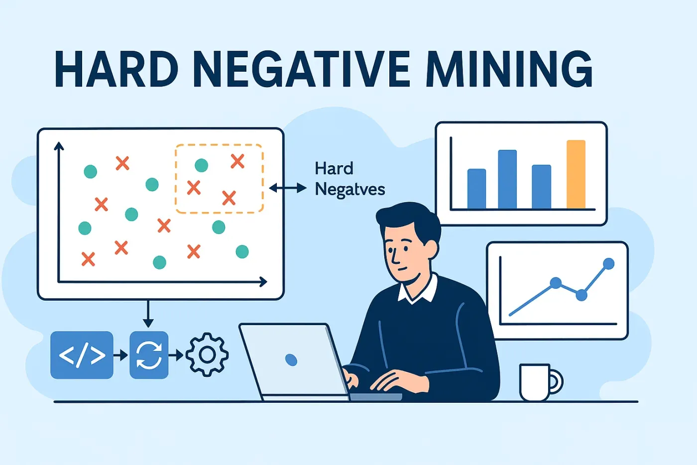
Hard Negative Mining: A Practical Guide for Senior Developers
Machine learning models - especially those used in search, recommendation systems, and computer vision - often fail not because they lack data, but because they lack the right data. One of the most powerful techniques to improve model robustness is Hard Negative Mining, a strategy that deliberately focuses the model on the most confusing, high-value mistakes.
If you’re building embeddings-based search, ranking systems, contrastive models (Siamese, Triplet, CLIP-like), or classifiers that struggle with look-alike examples, hard negative mining may be what you’re missing.
This post walks through the idea, why it works, real-world applications, implementation patterns, and pitfalls.
What Is Hard Negative Mining?
Hard Negative Mining (HNM) is a method for selecting the most challenging incorrectly-predicted samples and using them to train your model. Instead of training on random negatives (easy negatives), the model learns from:
- Hard negatives: samples that look very similar to positives
- Semi-hard negatives: samples that are close in feature space but still correctly classified
- False positives / ranking errors: negatives incorrectly ranked above the true positive
Hard negatives expose confusion patterns and force the network to sharpen its internal representations.
Why It Matters
Most real-world datasets are full of “easy negatives” - examples that are obviously different. Training on them provides little value.
Example: A face recognition model easily distinguishes:
- Barack Obama → positive match
- A dog → easy negative
But it struggles with:
- Barack Obama vs. Denzel Washington → hard negative
Without exposing the model to such pairs, it learns shallow features.
Hard negatives improve:
- Embedding separation (for vector search, retrieval)
- Classification boundary clarity
- Generalization on unseen data
- Model robustness to look-alike or noisy inputs
How Hard Negative Mining Works
1. Baseline training. Start by training the model normally using available data.
2. Identify hard negatives. During or after training:
- Compute embeddings
- Compute similarity scores
- Find samples incorrectly ranked above true positives
- Select top-K most confusing negatives
This is often implemented using distance metrics like cosine similarity or Euclidean distance.
3. Re-train / fine-tune. You feed the model:
- (anchor, positive, hard negative) → for triplet loss
- (positive, hard negative) → for contrastive losses
- mislabeled/confusing images → for classifiers
4. Iterate. Hard negative sets evolve as the model improves, so mining is often refreshed periodically during training.
Common Use Cases
Visual search / image retrieval. E-commerce models confuse similar shoes, T-shirts, or furniture. Hard negatives often improve ranking precision significantly, especially among visually similar items.
Face recognition. FaceNet popularized semi-hard triplet mining: negatives are picked inside the batch so they are hard, but not impossibly hard. ArcFace takes a different route entirely - a margin-based classification loss instead of explicit negative mining. The contrast between the two is a useful reminder that mining is one tool for separating embeddings, not the only one.
NLP and embeddings. With sentence-transformers, hard negative pairs help models distinguish:
- “refund policy” vs. “shipping policy”
- “invoice number” vs. “order number”
Recommendation systems. Embedding-based recommenders learn user/item vectors; hard negatives help with:
- look-alike items
- items purchased together
- items from the same category
Audio matching. Learned audio embeddings (cover-song detection, music tagging) use hard negatives such as tracks with similar spectral features. Classic fingerprinting systems like Shazam are a different beast - spectral hashing rather than trained embeddings - so mining does not apply there.
Implementation Patterns
Pattern 1: Offline Hard Negative Mining
You compute negatives once before training.
Pros: simple, scalable Cons: static, may not reflect model evolution
Code-style pseudo-example:
for anchor in dataset:
    pos = anchor.positive
    embedding_anchor = model(anchor)
    distances = compute_similarity(embedding_anchor, all_embeddings)
    hard_neg = pick_top_k_negatives(distances)
    training_pairs.append((anchor, pos, hard_neg))
Pattern 2: Online Hard Negative Mining (In-Batch)
The model identifies hard negatives dynamically during each batch.
Used in:
- CLIP
- SimCLR
- FaceNet (semi-hard mining)
Pattern 3: Dynamic Memory Bank
Large-scale setups (billion-scale search engines) use memory queues to fetch hard negatives across many batches.
Inspired by:
- MoCo (Momentum Contrast)
- Deep Metric Learning frameworks
Benefits & Pitfalls
Benefits
- Higher accuracy in embedding-based tasks
- Reduces overfitting to easy negatives
- Improves ranking metrics (NDCG, mAP, Recall@K)
- Makes contrastive models converge faster
Pitfalls
- Overly hard or mislabeled negatives can destabilize training. If negatives are impossible or mislabeled, the model can diverge.
- Computationally expensive. Mining requires large similarity computations.
- Needs well-curated positives. Garbage positives → unreliable negatives.
Summary
Hard Negative Mining is one of the most impactful techniques for improving ML models when data is abundant but easy. It forces models to learn deeper semantic distinctions by confronting them with confusing, meaningful mistakes.
Introduce HNM when:
- your embeddings cluster too close together
- search results occasionally return “almost correct” distractors
- classifier accuracy plateaus
- you scale up retrieval/recommendation systems
Combined with contrastive learning and modern embedding models, it is usually the cheapest way to buy back precision you thought required more data.